Owing to the width of most of the many data tables on this site, it is best viewed from a desktop computer. If you are on a mobile device (phone or tablet), you will obtain a better viewing experience by rotating your device a quarter-turn (to get the so-called “panorama” screen view).
The Owlcroft Baseball-Analysis Site
Baseball team and player performance examined realistically and accurately.
You can get a site directory by clicking on the “hamburger” icon () in the upper right of this page.
Or you can search this site with Google (standard Google-search rules apply).
Search term(s):
Analysis Basics
“‘Where shall I begin, please, your Majesty?’ he asked. ‘Begin at the beginning,’ the King said, gravely, ‘and go on till you come to the end: then stop.’”
It gets called a lot of thing: analysis, analytics, sabermetrics, and (by some traditionalists) a number of unprintable names. But a lot of things that analysts—most of them, anyway—would not call “analysis” are shoved into that category by the less-well-informed (including a lot of people professionally associated with the game) just because they involve numbers. Let’s clarify that.
Things like pitchers’ pitch spin rates, batters batted-ball “launch angles”, and fielders’ positioning (“shifts”) are all too commonly lumped into what is nowadays called “analytics”. Analytics they may be: analysis they are not. They are important, interesting, and useful things to know about, and when intelligently used can help a team to perform better. But so can strength training, aerobic exercise, good diets, and many, many other things, none of whch anyone is likely to refer to as analytics or as analysis.
Those sorts of things—analytics— wrongly lumped in with analysis are, without doubt, included simply because they deal in accumulated data, usually numeric. One could, it must be supposed, refer to acquiring and using such data to help improve player performance as “analyzing” the game, but that is really, really stretching the term. What such things are is coaching tools. Using such data is a wise and honorable thing to do, but it isn’t analysis. So…what is real analysis then? We’re glad you asked.
At bottom, it is the application, grounded in demonstrable success, of ways of applying stochastic mathematics† to numerical data—player and team statistics—to see how the various elements of the game combine to generate runs and wins. Nowadays, complicated measures with cryptic names (and, often, little explanation of their exact mechanics) have proliferated, to the confusion of those not already well grounded in these arts. It is our contention that the basic ideas, and even the basic “formulas”, are not at all difficult to grasp, and we will try to demonstrate that on this page.
(†Stochastic: from The Oxford Pocket Dictionary of Current English, “randomly determined; having a random probability distribution or pattern that may be analyzed statistically but may not be predicted precisely.”)
If you haven’t much background in mathematics, don’t worry. Some of the more advanced aspects of analytic investigation do call on what, for most, is arcane, but the basics require little beyond arithmetic.
What is a “formula”? It is an “equation”. And what is an equation? It is simply an assertion that one thing is equal to another thing, set down in mathematical form. If you go into a stationery-supply store to buy several pencils, all of the same kind, how much will it cost you? That depends on two things: the price of a pencil, and the number of pencils you will buy. Your cost (here we ignore complications like sales taxes) will be the price per pencil multiplied by the number of pencils. We can set that down in mathematical form as an equation, where we equate the cost with the price times the quantity:
Cost = Price x Quantity
Normally, though, one abbreviates, to keep things looking clean, so that might instead be written something like this:
C = P x Q
There: wasn’t that easy?
In baseball analysis, we develop various equations, with the left side being perhaps something like runs scored or games won, while the right-hand side is some set of baseball stats in some combination. We get those equations—those equalities—from a combination of logic and examination of history. And, as always in science (and this is science), we then submit our proposed equations to rigorous testing against massive amounts of real-world data.
But at this point, we need to take a little detour to discuss the nature of “baseball equations”. After all, no one is saying that some formula for, say, runs scored is always and ever and always going to give the exact number of real-world runs scored. So what use are these equations, and what does “testing them” mean? (This is where the “stochastic” part comes in.) We answer those questions next.
Baseball-related equations are probabilistic equations. What does that mouthful mean? Well, there are two basic kinds of equalities in the world: exact and probabilistic. An exact equation asserts something that we believe is always and ever exactly so; the distance a car will travel down a road is its speed (assuming for simplicity that we hold that constant) times the length of time it is driven:
D = S x T
Distance driven equals speed multiplied by time. That is exact: do 60 mph for two hours and you will always and ever cover 120 miles, exactly (or as exactly as we care to measure the distance, the speed, and the time). What other sort of “equality” could there be? A probabilistic “equality”. If you’re not used to thinking in such terms, that may sound abstruse, but fortunately easily understood everyday examples abound (since the universe we live in is ruled by probability).
Our first tool is nothing more complicated than a coin. We all know that an unbiased coin (meaning one not bent or scraped or very heavily engraved on one side only) comes up heads half the time and tails half the time: that is why we use coin tosses to settle so many things. But what is it that we “know” so surely? No one believes or expects that if you toss a coin over and over that it will come up heads-tails-heads-tails and so on forever; of course not. What we “know” is that as we toss a coin more and more, the percentage of heads (or tails) that we get will tend to get closer and closer to 50%.
If we toss a coin ten times and get 6 heads, we think absolutely nothing of it. If we toss the coin 100 times and get 60 heads, we notice it. If we toss it 1,000 times and get 600 heads, we are profoundly suspicious that it isn’t an unbiased, honest coin. And did we toss it 10,000 times and get 6,000 heads, we would consider that iron-clad proof that something is wrong with the coin. None of that is abstruse or mystic: it is founded in our ordinary experience of life.
We can write a very simple equation for heads in coin tosses:
H = T x 0.5
That says that heads come up as one-half of tosses. That assertion, that equation, is the one that we just said everyone knows is true; but we also said that everyone understands that it asserts something that is the long-term result of many trials— and that the more trials, the more nearly exact its results are, and correspondingly the fewer trials, the larger we expect the differences between its predictions and real-world results would be.
That is what a “probabilistic” equation is. No one is going to toss a coin 162 times, get 77 heads (or 84 heads) and announce that this heads-from-tosses equation is all a lot of hooey. But if a games-won equation says a given ball club is “a .500 club” and they win 77 or 84 games, some people will say that that equation is all just hooey. Obviously, we need some sort of yardstick to decide whether real-world results differ from what a probabilistic equation predicts by so much as to seriously question its validity, or whether they support the claim that it is “correct”.
Fortunately, the wonderful ways our universe works provide easy yardsticks for such testing. Here, we will just present the facts, but, one, you will find that they match ordinary intuition, and two, you can look up the details in many, many places (including a fairly technical article in Wikipedia).
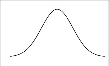
The intuitive relation we cited earlier, where we saw that the more trials (say, coin tosses), the closer we expect results to follow a prediction, happens to be an exact one. That that is so is one of the wonders of our cosmos—that “random” events follow very definite patterns of occurrence—but so it is. The general shape of the relation looks like this:
(Because the curve looks something like a cross-section of a bell, it is often just called “the bell-shaped curve”; its proper name is “Gaussian distribution” or “Normal Distribution”.)
What the graph above shows us is (this is simplified) the likelihood of the results of a given set of trials being just what is “expected”. The horizontal is the value of the result (say, for example, the number of heads in a given set of coin tosses), while the vertical is the number of trials that got that particular result. The peak at the center is just what is “expected” (in our example, 50% heads). Exact correspondence is the most likely result, with differences from that exactness becoming less and less likely as they become bigger and bigger. Wikipedia has a very nice animated display of this, which we reproduce below; in it, we see how the fit to the curve becomes better and better as we take more an more samples (in that image, n is the number of samples taken). Give the animation a few seconds to run through its paces from its start at n = 4.
As the number of discrete events increases, the function more and more resembles a normal distribution.
To try to ground this in familiar terms, let’s say that we toss a coin 162 times and record how many heads we got. Then we repeat that simple experiment many times. In the graph above, n is the number of 162-toss experiments we tried, and the dots sum up our results. The horizontal for a given dot is the number of heads, with 81 in the middle; the vertical is the number of 162-toss trials that had that many heads as a result. As you see, exactly 81 is the most frequent result, and the more we move away from 81—in either direction, higher or lower—the fewer and fewer trials give that result. And the more 162-toss trials we undertake, the more and more our results look like the expected curve.
To say much more would quickly take us into complexity, so we will just go with this takeaway: when we create a probabilistic equation, whether for heads in coin tosses or for runs scored from team stats, there are universally accepted standard tests for the predictions as compared to real-world results from real-world data, and those tests will tell us if our equation seems correct (or not). Those sorts of tests are used every day in everything from political polling to factory assembly-line quality-control sampling to nuclear physics.
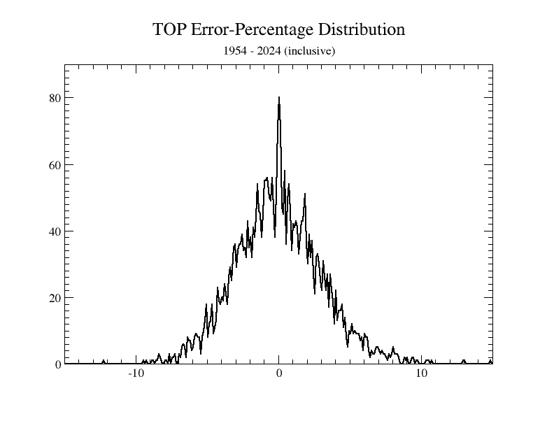
So that you can see if the Owlcroft run-scoring measure, the TOP, passes that test—a bell-shaped distribution of error percentages—we show the following:
Sure looks to us like a bell curve….
An interesting sidelight here is that added data become progressively less helpful in improving confidence. If a rookie bats .300 in his first full year, we are hopeful but not fully convinced; but if he bats .300 or so again the next year, we feel like the team has found a real .300 hitter. If he then bats .300 for his career—well, we already expected that, didn’t we? The increase in at-bats from the 1200 or so of his first two seasons to the perhaps 10 times as many of his full career gave us less new information than the mere doubling of the number from his first year to his second.
Mathematically stated, confidence goes up as the square root of the data multiple: that is, it takes four times as much data as we have to double our confidence in what those data are telling us. That’s one big reason why pollsters can determine pretty well, for example, how popular a given TV show is by surveying only a few hundred households.
For instance, if we do the math—which we won’t show here—using actual, historical numbers, we find that for 71 years of major-league baseball (1954 - 2024, inclusive), for runs scored we get an average variation from target of a little over 2 percent (just about 2.36%) from chance alone (that is using the TOP equation mentioned above, the most accurate one currently available). But over a more restricted period of time—say the first six weeks (one-quarter) of a season—the expected average scatter naturally rises (though by suprisingly little: the 2024 one-season average error was only 2.77%, compared to 2.36% for 71 seasons’ worth of baseball).
(We use 1954 as the start year because from 1953 to 1954 occurred the last change in official scoring rules, the restoration of the now-you-see-it-and-now-you-don’t Sacrifice Fly; that’s not a big factor, but it does make pre-1954 stats slightly incommensurable with those from prior years. And we’re measuring accuracy to a few hundredths of one percent.)
The point of this digression is that if you take the results of any competent analysis of baseball statistics—such as Owlcroft’s “TOP” formula—and repeatedly compare its predictions against real-world results, you expect to see a bell curve whose exact size and shape depend on definitely known numbers. If that is the case—and we showed above that it indeed is—you have good cause to say that the formula is correct. There are minor differences in accuracy between various different formulas from various different sources, but those differences are very small compared to the degree to which all of them, however derived by whom, generally agree with one another and with the expected scatter patterns probability mathematics demands of an accurate formula.
So that you can see that we put our money where our mouth is, we include a demonstration tabulation of the Owlcroft TOP formula tested on almost three-quarters of a century of major-league baseball stats. (You can also take a look at short-term results on the Team-Performance page on this site, but we don’t link it at this specific spot because you should read more before going there.)
Explaining this matter here would make this already long page far longer yet. The material is not terribly complex, but it is lengthy. We have thus moved it to a page of its own, The Games-Won Formula.
If we can—and we indeed can—project probable games won from runs scored and runs yielded over any arbitrary set of games (with, of course, increasing accuracy as the number of games in the series rises), we would next like to be able to project runs scored and yielded for a team based on who is playing and pitching for it. If we could do that as well—and here, too, we can—we could then project with some accuracy a team’s ultimate win percentage just from the identities of its player personnel.
(That assumes that we have enough history for each player to feel reasonably confident that we know his abilities well enough to use them in reckoning; we discuss that a bit more farther down this page.)
The essence of scoring runs in baseball is remarkably straightforward: put runners on base, then drive them in. The background is the ticking clock of baseball—outs. Of all the many and diverse numbers in baseball analysis, none is nearly so important as this one: three, the three outs that define an inning.
But to continue: another thing that probability mathematics tells us is that the chances of two things both happening is the chance for one multiplied by the independent chance for the other. To see a simple example of that that fact, imagine tossing a pair of standard six-sided dice, say one red and one green. What are the chances of getting a total of 5 showing?
The easiest way to see it is to use what mathematicians call a “Karnaugh Map”, which simply lays out all the possible combinations in a table, like so:
RED:
1
2
3
4
5
6
GREEN: 1
x
2
x
3
x
4
x
5
6
The little x’s show all the possible combinations that add up to 5. As you see, there are 4 of those; meanwhile, the total possible combinations are 6x6, or 36. So the chances of rolling a total of 5 are 4 in 36, which is 1 in 9, or 11.1%. Ta da.
Or, for another example, consider a two-engine plane for which we happen to know that the chances of either engine failing on a particular flight are 1% (one in a hundred). We also happen to know that the plane can be safely flown and landed with only one engine working, but that if both fail it will crash. What are the chances of a crash? They are one in ten thousand, or .0001 (or 0.01%, one percent of one percent). For a double fail, the first fail will only happen one time in a hundred; the second fail would have to happen in that one-in-a-hundred case, but only itself has a one-in-a-hundred chance. We won’t make the tedious Karnaugh map of 100 by 100 squares (10,000 squares), but if you imagine it, you will realize that only one of those 10,000 squares will be checked.
Now back to baseball.
The chance of a man getting on base is very simply expressed by a now-familiar (if late-arriving) stat: the on-base percentage. To get the chances of a man at the plate becoming a run scored, we need to take his on-base percentage and multiply it by some factor representing the chances that a teammate will knock him in. (We do need, naturally, to make some adjustment to the raw on-base percentage to allow for the facts that the man may get on by an error, and also that he may be put out on the basepaths even after having reached safely—Caught Stealing and Double-Play stats cover most but not all of such Outs On Base).
As an aside, we need to remember at all times—which many discussions and analyses we have seen do not—that the batter at the plate is also a base runner. That is, there is always at least one runner on for every batter: himself. He is the base runner on “zeroth base.” What he does as a batter independently affects him as a base runner (analysts sometimes forget that, but the Rules Of Baseball don’t, referring to the “batter-runner”). It is as if there are two men at the plate: a runner, just like a runner at any other base, and a batter who does what he does and then fades into thin air as the base runners (or runner—himself) do whatever is appropriate for what he as a batter did.
The mechanics of what such an “RBI factor” might comprise, and of how it is derived, are somewhat complicated. Evidently base hits are going to be very important, and extra-base hits especially so; but walks have some value, and even minor factors like hit-by-pitch and sac flies are not utterly negligible. In fact, the details of both the philosophy and practice of calculating an RBI factor of some sort are largely (but by no means wholly) what distinguish one school of analysis from another. Owlcroft has its own methods, which we will not detail here for a variety of reasons, most notably brevity.
In many workers’ formulations, the occurrence rate of Total Bases (the sum of all hits weighted by bases per hit—that is, for example, triples are 3 and singles are 1) is the only determinant in their RBI factor, whatever they call it (if they call it by a name at all). That can actually give a pretty fair result, and it has the virtue of simplicity. The first runs-scored formula (“Runs Created”) Bill James widely published was indeed that simple:
(Hits + Walks) x (Total Bases) / (At-Bats + Walks)
Since Hits + Walks is, roughly anyway, the available base-runner total, and At-Bats + Walks is—also roughly—the plate-appearances total, manifestly James’ “RBI Factor” in this formulation was indeed just the Total Bases rate (TB/PA, more or less). Note that James did not use the on-base percentage, or any rough equivalent of it: he used what amounts to the actual number of base runners. That’s OK for a quick, simple formulation which will serve to demonstrate how well analytic methods work, but it limits the utility of the formulation to evaluating what has happened; you cannot use it to predict what likely will happen because to know how many men will reach base, you need to state your formula in terms of an on-base rate. And that brings us to another important point.
The on-base percentage and an RBI factor, when multiplied, give the chance that a given batter will become a run scored; but the actual number of runs scored also depends on how many men come to the plate so as to have that chance. That number, actual total team plate appearances, varies significantly from team to team and year to year; but it does not do so without cause. Remember outs as the ticking clock of an inning: the less likely a team is to make an out at the plate, the more men they will get to the plate over the long haul.
That can be stated quite precisely in a mathematical formulation, but its essence for the purposes of understanding is this: a team’s on-base percentage has a form of “compound-interest” effect on run scoring. First, it directly increases the chance that any one batter will ultimately become a run scored; but second, it increases the number of men who will get to have that chance. It is for these reasons that the single most important baseball statistic viewed in isolation is the on-base percentage; actual run scoring tracks on-base percentage more closely than any other single statistic (as we now understand that it should).
Let’s construct a simple runs-scored equation, just to show the logic of the process; the one we now describe is one we published almost four decades ago, at which time we described it as “a very-much simplified version” of a full run-scoring equation. It looked like this:
       (H + BB) x TB
R = ―――――――――――――――――――― x G x 27 x 0.9430291185565
    (AB - H) x (AB + BB)
Let’s see what that breaks down into. As we noted above, H + BB is, roughly, men getting on base; also as noted above, AB + BB is, roughly, total plate appearances. TB is just Total Bases, which we are using as our “RBI Factor”. Beyond those, AB - H is (again, as always in this crude version, “roughly”) outs made. The G x 27 is simply all seasonal outs (which we approximate as 27 per game, not exactly true but quite close) times an empirical “fudge factor” (discussed in a moment) of about 0.943 (more exactly, 0.9430291185565).
Now let’s look at that equation in another way:
R = { (OB/PA) x (TB/PA) } x PA
The crucial point there is that the various PA values are not the same thing. The OB/PA and TB/PA figures use the real, actual PA value, because we need to know the rate at which OB and TB events happen. But the final PA is something different: it is the PA total that we expect from the OB/PA rate figure, and may well differ from the actual total.
(Of course, if all we want is to see what already happened, we can use the real, historical PA for all those values; but if we want to project the future, we need to use the historical rates but the projected PA total.)
The equation above is the simple idea stated above that the chances of a batter becoming a run are the on-base percentage (OB/PA) times an “RBI Factor” (here, simplified to just (TB/PA, the chances of a batter getting a hit) of one kind or another, and that runs are those chances of a man becoming a run times the number of men who actually get that chance (PA).
All we have done is to note that PA, plate appearances, is simply all available outs (roughly 27 x 162, or 4,374) divided by the chances of making an out, which is simply the outs rate, Outs per PA, which is just (AB - H)/PA). The rest—working the estimated PA’s into the basic equation—is just high-school algebra.
As we said before: there—wasn’t that easy?
Note that that equation uses only four stats: AB, BB, H, and TB (well, plus Games played, of course). The empirical part (that 0.0.9430291185565 multiplier) tries to roll up everything else, from men thrown out on the bases to sac flies and a ton more. Yet, for all the simplifying and ignoring that goes into such an elementary version, its accuracy over 1,828 team-seasons (every team for 1954 through 2024, inclusive) is an average error size of about 3.54% (exactly 3.5430494508143%), which compares decently with the full-force equation’s average error of 2.36%). It was and is remarkable how good one can get with even the simplest of formulas: four stats—and adding in everything else but the kitchen sink only gets us a bit over 1% better!
(What the “full” version does is introduce the complications: extra-base hits are weighted more accurately than the simplistic “1-2-3-4” weighting, things from walks to sac flies are introduced into the “RBI Factor”, each with an appropriate weighting, and suchlike. The mechanical details are messy, but the principles are simple and obvious.)
In that simplified four-stat formula we can, by “tuning” the weighting constants for the various hits that make up Total Bases (from that simplistic 1-2-3-4 basis), slightly improve the error size down to 3.49%. Then the increase in accuracy that going from just using four basic stats to the full range available would be only about 1.1% (3.49% to 2.39%). Obviously, the basic, simple idea captures most of what goes into run-scoring.
And one more time: if you have any doubts that the Owlcroft run-scoring equation works, and works very well, look over the actual results again.
Now consider this: what we can calculate for a team from its statistics, we can also calculate for any one batter from his personal statistics. If we then set the number of available outs to what it is for a full team for a full season, we get a number that sums up that man’s ability to contribute to his team’s scoring of runs in one number: we can think of it as the runs that would be scored in a season by a team made up entirely of exact clones of that man.
Owlcroft calculates just such a measure, which we also call the TOP (Total Offensive Productivity), just as we call it for teams. It is shown for all batters listed anywhere in these pages; in the by-team batting lists, the batters are arranged in order of descending TOP.
Moreover, what one can calculate for a batter, one can correspondingly calculate for a pitcher, using the numbers that he gives up to batters. You will find on this site just such calculations, which yield a novel and very, very important measure that we call the TPP, for Total Pitching Productivity, because the term pairs nicely with the TOP). We also generate a measure we call the “Quality of Pitching” stat, so those accustomed to using ERA as a measure can have something comparable to review. There is a separate page on this site that discusses those measures further, but you would be best off to finish this page before jumping there.
We need to have a care when thinking about player TOPs. A man’s value to his team depends on the other men on that team. That is because in reality the man is not in a batting lineup that is nine clones of him. The value of his OB percentage depends on the “RBI Factor” value of the men behinbd him; the value of his “RBI Factor” depends on the OB percentage of the men ahead of him. One way to better estimate his value might be to calculate for a lineup comprising him and eight imaginary league-average batters; but much would depend on (for just one thing) where in that order he would bat: the #9 batter gets only about 80% as many plate appearances as the #1 batter. A most interesting deduction from that truism is that the better the team, the less any one man means to its run-scoring, and the weaker the team, the more any one batter’s contribution matters. A corollary to that is that a team is better off with its batter TOP values evenly spread among its lineup than with them concentrated in a few top hitters. Better nine TOP 800 batters than four 900s, four 700s, and an 800. A key dictum in a paper we wrote for a major-league team for which we were consulting almost 40 year ago was Not all giants: just no midgets.
Two other somewhat related points need mention. (Actually, they need extensive discussion, and we hope in future, as we gradually expand these notes, to give them that discussion.) One—touched on earlier—is the predictability of individual men’s performances. As we said earlier, there is a law of diminishing returns for the meaning of increased data; by the time we have roughly the equivalent of two or at most three seasons’ full-time play for a batter, we have enough data to have defined his norms of performance tolerably well. Pitchers, for complex reasons, take more time to evaluate, although using the TPP instead of the ERA gives results in time periods comparable to those needed for batters. Moreover, by the time a batter reaches double-A ball, he has usually—not always, but usually—become pretty much what he will be; if we have two or three seasons’ worth of data above class A ball, we have the man fairly well defined. That is not true for pitchers, because batting is responsive, while pitching is initiative: a pitcher can, even late in his career, add a new pitch or other change to his delivery, whereas a batter can by and large only work with the reflexes nature has given him.
In the claims above, note well the phrase “full-time play”. Of late, some teams have been rushing young players up, usually out of desperate need. A man who has, over two seasons of above-Class-A ball might seem to fit the criteria for being a known quantity, but not when his grand total of games played for those seasons combined is 97; that’s not even the equivalent one one full season (plus it suggests that there may have been reasons for the low use, reasons that unfairly hurt his posted numbers). And such drastic jump-ups are no longer uncommon.
It is precisely that predictability that makes it possible to “engineer” a baseball team in a manner quite comparable to the process of engineering an automobile engine. By knowing the data for the components and the equations for how those components interact, we can design an engine or a team to meet a specified set of performance criteria.
It is crucially important to understand what we are saying here: we are not saying that we can predict accurately how every man will do in a given season from how he has done in the past; that is, as common sense suggests, impossible. But, just as we certainly cannot predict how a pair of dice will come up in any given throw or small number of throws—which is why people gamble—we can certainly predict with great accuracy how much money a craps table will likely take in on a shift because we know the tendencies of the dice. So with a ball club: if we know the tendencies of the batters and pitchers—what they have done in the past—we can predict with good accuracy how the cumulative results of 26 men over a full season will come out (and we do that on a page of the site). We know some men’s performances will be surprisingly low and some surprisingly high, but—most of the time—the team net will be close to the estimate. (A full season for a ball club is enough for acceptable precision, but there is always room for the occasional burst of especially good or bad luck called by most fans—as well as professionals who should know better—either “clutch performance” or “choking.” (How come no sane craps player ever refers to “clutch” dice or “choking” dice when they win or lose?)
The second point, related to what we just said, is that minor-league statistics—long thought by most baseball professionals and fans to be nearly meaningless—can be translated so that we see what the man would have achieved playing at that same level of ability in a major-league ballpark against major-league competition. (That realization, and the mechanics to implement it, are one of Bill James’ most valuable contributions—probably his most valuable—to the art.)
Finally, we repeat that all statistics, to be useful, must be comparable. There is a separate page on this site that discusses “normalization” processes for stats and why they have become a statistical nightmare (we no longer apply them, preferring honestly raw results to results “adjusted” by such dubiously derived factors).
A wholly other way of reckoning runs scored from a team stat line is something called “Linear Weights” (LW). It works on the implicit assumption that results from any one datum—say singles—affect run-scoring on a straight-line relation (hence “linear”), so that runs can be calculated by using a set of weighting constants (hence “weights”), looking something like this:
R = (k1 x 1B) + (k2 x 2B) + …
The various weighting constants can be gotten in many ways, mostly empirical. We can also, in principle, get them from a run-scoring equation of the probabilistic kind described farther above. We just lug in all-MLB-average team stats, then see what effect on the runs total comes up if we add one more, say, single (something often called the “plus-one” value). That, in principle, gives the weighting factor for whatever stat we plus-one’ed (such as singles).
How to do that isn’t as obvious as it might seem at first blush. Do we add one more PA and assign it to a single? Or do we change one existing out to a single? And either way, what about the change in the PA total that arises from improving the OB%? Points to consider.…
One issue we see with LW, which we method do not use or elsewhere refer to on this site, is that the value of, say, a single is not a fixed thing: it will mean more on teams with more power and higher OBPs, because a man who gets on has a better chance of scoring on such teams, and conversely less for weaker teams for analogous reasons. Some people love LW; we don’t. We prefer measures that have an underlying logic and are not 100% empirical.
Baseball Reference, in their explanation of Base Runs (another run-production method), remarks: research has shown that run scoring is not entirely linear. That is…the evidence suggests that at the team level, a linear conception of offense can break down at the extremes. If you check the graph for the TOP, you will see that it does not fail at the extremes of scoring.
Base Runs
Base Runs is, we feel, the only serious competitor to the Owlcroft TOP. On another page here, where we discuss the accuracy of the TOP and show it in a graph, we also compare it to Base Runs; click the link to see that comparison (it will open in a new browser tab). It will come as no surprise that the TOP is the better method, but Base Runs is pretty good (especially if one “tunes” the rather simplistic weighting constants usually shown in published versions of the equation).
The Alphabet Soup
As any modern baseball fan knows, there is also an entire alphabet soup of other metrics out there, from fWAR to UZR to xFIP and so on and so forth. These have value, some more than others, but there are two points about them as a class that especially bother us.
One is that many of them, notably the “WAR” stats (“Wins Above Replacement” if you didn’t know) is that they are not rate measures but cumulative measures. If I am thinking of buying a racing car, I mainly want to know how fast it goes; I am not especially interested in how many miles it drove in the last week or month or racing season. While if I were to examine its history I could probably derive, in time, its average speed in driving those miles, that is a roundabout way of getting to what should be a single, simple datum. I don’t care how many WAR a player has in a given season because I did not control (and may not know without some looking-up) how often the player played, and why he wasn’t playing when he wasn’t (hurt? platooned? manager’s dog house? something else?). And, of course, another issue is the entirely artificial and arbitrary “replacement-value” standard; back at the race-car analogy, do I care about miles driven in a racing season above those of some imaginary “replacement car”? Really?
A second issue, possibly even more pernicious, is that the modern alphabet soup is mostly or wholly relative measures. Things like games won or runs scored are results that correspond to real-world facts: we can (a) test any equations for them against real-world data and prove—or falsify—our hypotheses, and (b) easily understand and use those results. But with relative measures, we have slip-slided all the way back to pre-analysis days, when taverns were filled with baseball fans arguing over whether this guy’s batting average made him more valuable than that guy’s RBIs, and no real way (save having the louder voice) to settle the argument.
It was a very long uphill battle to establish credibility for analysis in baseball, and the war is far from over. To revert from real, absolute numbers to arcane and wholly relative measures just re-establishes in old-timers minds the idea that all this numbers stuff is just a fancified set of tavern arguments. Sure, an analyst can add up a team’s players’ and pitchers’ WARs and get a team number, but it’s a number founded on an entirely imaginary and arbitrary team of “replacement-value” players. “Find and point to that team, and show me in print that team’s wins,” might any baseball executive say. And what is the reply to be?
Having come this far on the site, you may be wondering where to look next. We recommend that before you cut to the daily data pages, you look over our detailed explanation of the various important data on our main Team Performance Tables page, so that the results we present there will have meaning for you.


 ) in the upper right of this page.